Incorporating Home Equity into a Retirement Income Strategies
by
Wade D. Pfau
Professor of Retirement Income at The American College
Director of Retirement Research, McLean Asset Management
Abstract
Strategic use of a reverse mortgage can improve retirement outcomes. The benefits are non- linear in nature, as they relate to the synergies created by reducing sequence risk for portfolio withdrawals and to the non-recourse aspects of reverse mortgages that can potentially allow a client to spend more than the value of their home. This article explores six different methods for incorporating home equity into a retirement income plan through the use of a reverse mortgage. Generally, strategies which spend the home equity more quickly increase the overall risk for the retirement plan. More upside potential is generated by delaying the need to take distributions from investments, but more downside risk is created because the home equity is used quickly without necessarily being compensated by sufficiently high market returns. Meanwhile, opening the line of credit and that start of retirement and then delaying its use until the portfolio is depleted creates the most downside protection for the retirement income plan. This strategy allows the line of credit to grow longer, perhaps surpassing the home’s value before it is used, providing a bigger base to continue retirement spending after the portfolio is depleted. Use of tenure payments or one of the coordinated spending strategies can also be justified as providing a middle ground which balances the upside potential of using home equity first and the downside protection of using home equity last. A key theme is that there is great value for clients to open a reverse mortgage line of credit at the earliest possible age.
Introduction
The use of a reverse mortgage to supplement portfolio withdrawals as a part of retirement income strategies is a fascinating topic and a number of counterintuitive findings are slowly entering into the financial planning profession. Since 2012, the Journal of Financial Planning has served as the primary outlet for a series of research articles demonstrating the potential use and value of reverse mortgages as part of a comprehensive retirement income strategy. The studies published in this journal could very well lead to the strategic use of home equity in a retirement income plan to become the next hot topic for client and advisor education, similar to how webinars and seminars about Social Security claiming strategies have been ubiquitous in recent years.
For most Americans, home equity and Social Security benefits represent the two biggest assets on the household balance sheet, frequently dwarfing the available amount of financial assets. Even for wealthier clients, home equity is still a significant asset which should not automatically be lumped into a limiting category of last resort options once all else has failed. It is a great shame for the financial planning profession that the conventional wisdom about reverse mortgages continues to remain so negative and to be based on so many misunderstandings about their potential uses.
Regarding the advances made in this journal, Sacks and Sacks (2012) led the way with their demonstration for how a strategy which coordinates draws from a reverse mortgage line of credit throughout retirement can significantly increase the probability of success relative to the conventional wisdom strategy that a reverse mortgage line of credit only be opened and used as a last resort option once other resources have been depleted. Salter, Pfeiffer, and Evensky (2012) and Pfeiffer, Salter, and Evensky (2013) followed suit, independently confirming how their coordinated glidepath strategy for home equity use could also increase the success probabilities for a variety of withdrawal rates. Wagner (2013) represents a fourth key study which garnered greater respect for the reverse mortgage term and tenure options in addition to draws from the line of credit. Pfeiffer, Schaal, and Salter (2014) later provided a more detailed analysis about two options using home equity last in retirement, with the difference being whether the reverse mortgage is opened early or when it is first needed. They found that establishing the HECM line of credit early is especially advantageous in low interest rate environments.
Despite the significant contributions found in these past studies, there is still room for another investigation of the government’s Home Equity Conversion Mortgage (HECM) program. This study aims to bring further clarity to what these past studies found by pushing deeper into the underlying analysis about how these strategies impact spending and wealth. Past studies have generally struggled with how to explain the combined impacts of home equity use on sustaining a retirement spending goal as well as preserving assets for legacy. When describing the impacts on legacy, past articles have generally focused on the median amount of legacy wealth and struggled with how to make proper comparisons in cases when the full spending goal was not met. One objective for this article is to focus on the wider distribution of potential outcomes to better understand the combined impacts for spending and legacy.
Past studies have also struggled with how to simulate the random future fluctuations for all the key variables which will impact the results. While past studies have employed Monte Carlo simulations for stock and bond returns, none of these studies simulated the future paths of interest rates, nor did they link future bond returns to future interest rates. This misses the ability to see how changing interest rates impact line of credit growth, the amount of credit available when delaying the decision to open a reverse mortgage, and the interplay of growth in the line of credit or loan balance for the reverse mortgage and the return on bonds in the investment portfolio. While some studies also provide scenario testing with regard to whether interest rates are fixed at high, medium, or low levels in the future, the present study allows a deeper analysis by simulating interest rates and linking them to future bond returns.
As well, this study also provides random simulations for future home prices, while past studies have used a fixed growth assumption for future home prices. Home prices are another key variable because they impact the amount of credit available when delaying the option to open a line of credit, and because home prices are a pivotal piece of the puzzle to determine whether the non-recourse aspects of reverse mortgages will become binding.
To be clear, the combined effects of future market returns, future interest rates, and future home prices tend to work together in rather complicated ways because of some nonlinearities existing with the use of a reverse mortgage. By simulating all the relevant variables, this article seeks to help make greater sense about how reverse mortgage strategies can work in a retirement income plan.
When given a choice for meeting a particular year’s spending goal using either a portfolio withdrawal or using a draw from the reverse mortgage line of credit, the ultimate impact on legacy wealth is unknowable in advance. The best we can hope to do is to study the distribution of outcomes with different strategies and then choose the strategies with which we are most comfortable with in terms of the combined impacts on spending and legacy. Choosing the portfolio as the spending source will impact the ultimate legacy amount in a random way which depends on the realized market returns that spending would have experienced in the subsequent years of retirement had it stayed in the portfolio. The opportunity cost of portfolio spending is whatever market returns (good or bad) it would subsequently experience. The impact of spending from the reverse mortgage line of credit relates to how future interest rates will impact the ultimate loan balance due. Could assets left within the portfolio grow more quickly than the reverse loan balance? To answer this question fully requires introducing an important non-linearity. A reverse mortgage is a non- recourse loan. Should the loan balance ultimately exceed 95% of the appraised value of the home when payment is due, which Pfau (2014) demonstrates is a reasonably likely outcome for retirements starting when interest rates are low, then the ultimate legacy reduction impact of some home equity draws could be $0. The likelihood that this happens depends on both the random path of future interest rates and future home prices.
Another important non-linear aspect of home equity use is the synergetic aspects which can be created through its treatment as a buffer asset to mitigate sequence of returns risk for the retirement portfolio. Bengen (1994) ushered in the modern study of sustainable withdrawals from investment portfolios within the realm of financial planning. His 4% rule came about as the answer to which initial spending rate, which provides a spending amount that is subsequently adjusted for inflation, could be sustained historically for 30 years from an investment portfolio with 50-75% stocks. His study provides a research simplification which has guided much subsequent research, though it must be clear that this constant inflation-adjusted spending from a volatile investment portfolio is a unique cause of sequence of returns risk in retirement. This is why the 4% rule is the 4% rule. Even when the average market return over a 30-year period is reasonable, the sustainable spending rate can still be low if a poor sequence of market returns is experienced early in retirement. This pushes up the withdrawal rate as a percentage of the remaining lower balance required to continue meeting the spending goal, which creates a hole for the portfolio and prevents it from growing even when the overall markets subsequently recovers.
If spending is allowed to decrease in response to poor market returns, this mitigates sequence risk by reducing the spending percentage relative to what is left. Alternatively, overall spending does not necessarily have to decrease if part of the spending goal can instead be covered through an alternative buffer asset. This is where the reverse mortgage fits into the puzzle. Reducing portfolio draws when markets are down by sourcing that spending from elsewhere is another effective method for mitigating sequence risk. That sequence risk reduction is the source of the synergy and is precisely the objective of the coordinated spending strategies developed by Sacks and Sacks (2012) and Salter, Pfeiffer, and Evensky (2012).
For these reasons, when using Monte Carlo simulations to study different coordinated spending strategies in retirement, there will not be one superior strategy. Sometimes strategies which use up the reverse mortgage line of credit as quickly as possible will perform best. In other cases, strategies which delay home equity use for as long as possible will be proven the winners. As well, coordinated strategies which draw occasionally from a line of credit will frequently can also do well. Even more, strategies which systematically use home equity through retirement by creating a tenure payment may perform best. The objective for this article is to analyze these different possibilities in order to provide planners and their clients with a deeper context for considering how to incorporate home equity into a retirement income strategy.
Overview of the HECM Reverse Mortgage Program
There are a number of available overviews about the HECM reverse mortgage program. The government frequently modifies program rules, which does mean that anything written before September 2013 will be describing conditions rather different from today. At that time the government streamlined the program to offer a single HECM option, eliminating what had previously been two options: the HECM Standard and HECM Saver. More recently, new safeguards have been created to reduce the initial amount of available credit, to protect non-borrowing spouses who are under 62 when a reverse mortgage begins, and to provide financial assessments to assure that borrowers will be able to meet the requirements for property taxes, insurance, and home maintain to keep the mortgage from foreclosing. Johnson and Simkins (2014) provide an excellent and up-to-date introduction. Giordano (2015) also provides a comprehensive treatment for how the HECM program works.
Reverse mortgages have a relatively short history in the United States. The first was offered by a bank in Maine in 1961. In 1989, the federal government systematized reverse mortgages through the Home Equity Conversion Mortgage (HECM) Program under the auspices of the department of Housing and Urban Development (HUD). In recent years, HUD frequently updated the administration of the HECM program to help ensure that any problems are corrected and reverse mortgages are used responsibly. The basic objective is to create liquidity for the home value so it can be used more efficiently in retirement.
Eligibility
Requirements to become an eligible HECM borrower include age (at least 62), equity in the home (any existing mortgage can be paid off with loan proceeds), financial resources to cover tax, insurance, and maintenance expenses, no other federal debt, competency, and the receipt of a counseling certificate from an Federal Housing Authority (FHA) approved counselor for attending a personal counseling session on home equity options. The property must serve as the primary residence and also must meet FHA lending codes and pass an FHA appraisal to be eligible. Up to $625,500 of a home’s value can be applied to a reverse mortgage.
Initial Available Credit
The important factors for determining how much credit is available through the HECM include the appraised home value, the age of the younger spouse (for joint owners, one spouse must be at least 62), a lender’s margin, and the 10-year LIBOR swap rate. Together, the lender’s margin and 10-year swap rate sum to the “expected rate.” This is used with the age of the younger spouse to determine the principal limit factor (PLF), or the percentage of the home’s value that may be borrowed. For the example described in the methodology section, the initial available credit is 52.4% of the home’s value.
Upfront Costs
When the line of credit is opened, fees include a 0.5% upfront mortgage insurance premium payment (when first year borrowing is less than 60% of the line of credit, which will be the case for all scenarios in this article), loan origination fees, and other closing and settlement costs. These fees can be paid in cash, or they can be borrowed from the available line of credit. Recently, lenders have been providing more options regarding the acceptance of a higher margin rate accompanied by lower origination costs and the ability to have ongoing service costs covered by the lender’s margin.
Ongoing Credit and Loan Balance Growth
Once determined through the PLF, the principal limit which can be borrowed against will grow automatically at a variable rate equal to the lender’s margin, a 1.25% mortgage insurance premium (MIP) and subsequent values of 1-month LIBOR rates. Any outstanding loan balance also grows at this rate. As well, the line of credit almost always grows at this rate, with rare exception when there are set asides for servicing costs growing at a different rate. Those exceptions do not apply herein, so that total principal limit, loan balance, and remaining line of credit all grow at the same variable rate. The total principal limit equals the sum of the loan balance and the remaining line of credit. Once enough is borrowed so that the loan balance equals the principal limit, no further borrowing is possible except if a tenure payment was chosen or if some loan balance is repaid.
These LIBOR rates are the only variable part for future growth, as the lender’s margin and MIP are fixed at the beginning. A key feature of the HECM program is that it is a non- recourse loan. No matter how much is borrowed, the amount due cannot exceed 95% of the home’s appraised value when repayment is due.
Spending Options
For the adjustable rate versions of HECM loans most commonly used today, the proceeds from the reverse mortgage can be taken out in combination of any of these four ways:
- Lump-sum payment: take out a large amount initially, though not necessarily the full amount available, perhaps to pay off existing mortgage or to use as HECM for Purchase.
- Tenure payment: works similar to an income annuity with a fixed monthly payment guaranteed to be received for as long as the borrower lives and remains in the home.
- Term payment: a fixed monthly payment is received for a fixed amount of time
- Line of Credit: home equity does not need to be spent initially, or ever. A number of strategies involve opening a line of credit and then leaving it to grow at a variable interest rate as an available asset from which to draw to cover a variety of contingencies later in retirement
Though portions of the loan balance may be repaid without penalty at any time, the loan balance does not have to be repaid until the borrower (and eligible non-borrowing spouse, when applicable) have left the home, either through death or by moving. Heirs can then generally arrange to have up to 12 months to repay the loan balance, or to otherwise hand over the keys to the home and walk away if they believe the loan balance is significantly higher than the appraised value and the potential selling price for the home. The loan balance can be repaid by selling the home, though heirs wishing to keep the home within their family could repay the loan balance with other funds or by seeking a traditional mortgage to refinance the reverse mortgage.
Tax Matters
Any distributions from the HECM are treated as loan receipt and are not taxable. Distributions from the HECM are not included in the Adjusted Gross Income, which may help with tax bracket management and may impact the taxation of other government benefits in retirement. When the loan balance is repaid, heirs might have to pay taxes on any non-recourse funds received in excess of the home’s appraised value. Heirs may also be able to tax a large interest deduction for the portion of the repaid loan balance which covers interest due. A tax professional should be consulted for more specifics on a particular client’s case.
Methodology
I simulate reverse mortgage strategies using 10,000 Monte Carlo simulations for 10-year bond yields, equity premiums, home prices, short-term interest rates, and inflation. Stock and bond returns are calculated from simulated bond yields and equity premiums above bond yields. The details of the underlying market simulations are provided in the appendix.
These simulations reflect the lower bond yields available to retirees today, but they do include a mechanism for interest rates to gradually increase over time, on average. Bond returns are calculated from the simulated interest rates and their changes, and stock returns are calculated by adding a simulated equity premium on top of the simulated interest rates. All strategies will be simulated with the same asset allocations and portfolio returns in order to make the results comparable. Strategies are simulated with annual data, assume withdrawals are made at the start of each year, use annual rebalancing to restore the targeted asset allocation, and no fees are deducted from remaining portfolio assets at the end of the year. Without much loss of generality, this also requires assuming that home equity draws and growth in the principal limits and loan balances are calculated annually instead of monthly. An annually rebalanced asset allocation of 50% stocks and 50% bonds is used so that greater emphasis can be made on exploring different uses for home equity.
In October 2015, the 10-year LIBOR Swap Rate was 2.01% and the 1-month LIBOR rate was 0.2%. Assuming a 3% lender’s margin rate, this leads to an expected rate of 5.01%, which translates into a principal limit factor of 52.4% for our assumed 62-year old borrower. For the baseline study, I assume a home value of $500,000. At loan origination, this requires an initial mortgage insurance premium of 0.5%, or $2,500. I assume that other origination and closing costs combine for a total initial cost of $5,000 when the loan is initiated. Except for the strategy in which the line of credit is drawn down first before spending from the investment portfolio, I assume that this initial cost is withdrawn from the portfolio rather than added to the loan balance. The initial effective rate for principal limit growth adds the 0.2% 1-month LIBOR rate to the 3% margin and the 1.25% ongoing mortgage insurance premium, which is 4.45% initially. This is a variable rate which will subsequently fluctuate based on simulated short-term interest rates.
The client holds a $1 million portfolio in a tax-deferred investment portfolio. In order to provide a basic understanding about the impact of taxes, a marginal tax rate of 25% is applied to any portfolio distributions. Distributions from the HECM reverse mortgage do not require any tax payments. The withdrawal rate reflects post-tax inflation-adjusted spending goals as a percentage of the initial portfolio balance. For instance a 4% withdrawal rate represents $40,000 of spending from the $1 million portfolio. The spending amount subsequently grows with the simulated inflation rate. If this distribution is taken from the portfolio, the withdrawal in real terms is $40,000 / (1 – .25) = $53,333 to cover taxes as well. If taken fully from the HECM, only $40,000 is needed.
Within each simulation, home prices grow randomly, and the HECM line of credit grows randomly in response to changing short-term interest rates. In each simulation, spending is sourced from the appropriate asset as based on the rules for that strategy. When a strategy calls from spending from a depleted asset (the financial portfolio or home equity), the other asset is used instead when still available. Once both assets are depleted, shortfalls below the spending goal are tabulated in order to provide a negative legacy wealth value. This is the real value of the spending shortfall without any applying any investment returns or discount rates. Doing this is important to reflect the magnitude of failure with a strategy. Legacy wealth is calculated as the remaining portfolio balance plus any remaining home equity at the end of retirement. Remaining home equity is calculated as 95% of the home’s value at the end of retirement less any balance due on the reverse mortgage loan. Because of the non-recourse features of the HECM program, remaining home equity cannot be negative, even if the loan balance exceeds the home’s value.
Seven total retirement income strategies will be considered, six of which involve spending from a HECM:
- Ignore Home Equity: This is the only strategy which is not comparable with the others, as it makes no use of the home equity. The strategy is only used to indicate a baseline probability of plan success when home equity is not used.
- Home Equity as Last Resort: This strategy represents the conventional wisdom thinking regarding home equity. It is the only home equity strategy which delays opening a line of credit with a reverse mortgage. The investment portfolio is spent first. If and when the portfolio is depleted, a line of credit is opened with the reverse mortgage and spending needs are then met with the line of credit until it is fully used. The PLF is calculated using the current PLF table for the updated age and simulated interest rate value at the future date, assuming the same underlying 3% margin rate.
- Use Home Equity First: This strategy opens the line of credit at the start of retirement, and retirement spending is covered from the line of credit first until it is fully used. This allows more time for the investment portfolio to grow before being used for withdrawals after the line of credit is depleted.
- Sacks and Sacks Coordination Strategy: This strategy opens the line of credit at the start of retirement, and spending is taken from the line of credit, when available, following any years in which the investment portfolio experienced a negative market return. No efforts are made to repay the loan balance until the loan becomes due at the end of retirement.
- Texas Tech Coordination Strategy: This strategy is modified from the original strategy described in Pfeiffer, Salter, and Evensky (2012) to remove the cash reserve bucket. This strategy performs a capital needs analysis for the remaining portfolio wealth required to sustain the spending strategy over a 41-year time horizon. Spending is taken from the line of credit when possible, whenever the remaining portfolio balance is less than 80% of the required wealth glidepath. Whenever investment wealth rises above 80% of the glidepath value, any balance on the reverse mortgage is repaid as much as possible without letting wealth fall below the 80% threshold, in order to keep a lower loan balance over time and provide more growth potential for the line of credit. The line of credit is opened at the start of retirement.
- Use Home Equity Last: This strategy differs from the “home equity as last resort” strategy only in that the line of credit is opened at the start of retirement. It is otherwise not used and left to grow until the investment portfolio is depleted.
- Use Tenure Payment: This strategy opens the line of credit at the start of retirement and uses the tenure payment strategy. With an initial home value of $500,000, an expected rate of 5%, and an age 62 start, annual tenure payments from the line of credit are $17,972. Any remaining spending needs are covered by the investment portfolio when possible.
Results
Results are presented for an each strategy assuming an asset allocation of 50% stocks and 50% bonds. Results are displayed for years in retirement, allowing the retirement duration to be interpreted either as the date of death for the client, or at the date in which the client leaves their home and must repay the reverse mortgage loan balance. Though it should really only represent a starting point for the analysis, since it considers only one point in the distribution of outcomes, Figure 1 shows the probability that the expenditure objectives for a 4% post-tax initial spending rate can continue to be met as retirement progresses. With a 25% marginal tax rate, this would imply a gross withdrawal rate of 5.33% in the first year of retirement if distributions are taken solely from the investment portfolio.
Figure 1
Probability of Success for a 4% Post-Tax Initial Withdrawal Rate
$1 million portfolio, $500,000 home value, 25% Marginal Tax Rate

For this figure, a strategy which ignores home equity is included as a reference point, though it is not directly comparable with the others since home equity is not used to support retirement income. With higher expenditures to cover taxes as well, the baseline shows that the success rate for the retirement spending goal is only about 40% by the 30th year of retirement.
The other strategies are all comparable, because they all allow home equity to be used to meet spending goals as well. Of the six strategies which use home equity, the strategy supporting the smallest increase in success is the conventional wisdom of using home equity as a last resort and only initiating the reverse mortgage when it is first needed. This confirms Sacks and Sacks (2012) original finding. Meanwhile, the strategy which uses home equity as a last resort, but which opens a line of credit at the start of retirement in order to let the line of credit grow before being tapped, provides the highest increase in success rates. Especially when interest rates are low, the line of credit will almost always be larger by the time it is needed when it is opened early and allowed to grow, than when it is opened later. Meanwhile, the benefits from the other four strategies fall somewhere in between. Success rates increase as one adjusts from using home equity first, to using the tenure option, to using either of the coordination strategies.
The basic understanding derived from Figure 1 is that strategies which open the line of credit early, but then which delay its use for as long as possible will offer increasing success rates as more line of credit is available to be drawn from if and when it is eventually needed. This benefit from delay is sufficient to counteract the reduced sequence risk created by using the line of credit in a more coordinated way over time.
But the probability of success is not the only relevant measure for outcomes. Importantly, clients may be concerned about the combined legacy value of their assets when using a reverse mortgage. Legacy value is defined by any remaining portfolio assets plus any remaining home equity after the reverse mortgage loan balance has been repaid. When assets were depleted (the portfolio and the entire line of credit), legacy values are counted as negative by summing the total spending shortfalls which would manifest either as reduced spending or as a need to rely on ones’ heirs for additional support while alive as a form of “reverse legacy.” Any taxes to be paid by heirs are not included in the numbers show for the next three figures which examine the range of legacy values. These figures are shown for the six strategies which do incorporate home equity, so they are all comparable.
Figure 2
Median Real Legacy Value for a 4% Post-Tax Initial Withdrawal Rate
$1 million portfolio, $500,000 home value, 25% Marginal Tax Rate
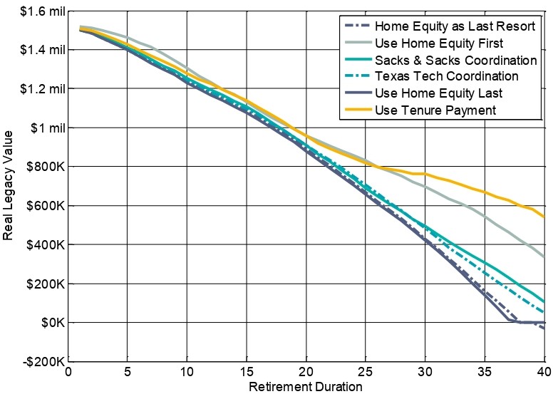
First, median wealth outcomes are most comparable to what has been shown in previous research, though past articles have struggled to make results comparable by not accounting for negative legacy values when there are spending shortfalls. What we can observe in Figure 2 is that median legacy values remain close for the first 20 years of retirement, with spending home equity first providing the highest legacy value and spending home equity last provides the smallest legacy value. For the median outcomes, the investment portfolio grows more quickly than the outstanding loan balance on the reverse mortgage, so that clients are served best by preserving their portfolio as much as possible while spending down home equity first. As retirement progresses, after about 25 years, the legacy value for the tenure payment option changes slope and starts supporting significantly more legacy. This is a combined result of the partial home equity use preserving the portfolio longer, as well as the fact that eventually tenure payments enter into the non-recourse aspect of the reverse mortgage, as the income continues for as long as the client is in their home even if the loan balance has already exceeded the line of credit. It is the only HECM option which allows this. The other important observation to make from this figure is that legacy values become level at $0 when home equity is used last, as these reflect situations in which spending is still possible from the line of credit, though the line of credit has already grown to be worth more than the home. Such spending has no impact on legacy.
Figure 3
90th Percentile Real Legacy Value for a 4% Post-Tax Initial Withdrawal Rate
$1 million portfolio, $500,000 home value, 25% Marginal Tax Rate
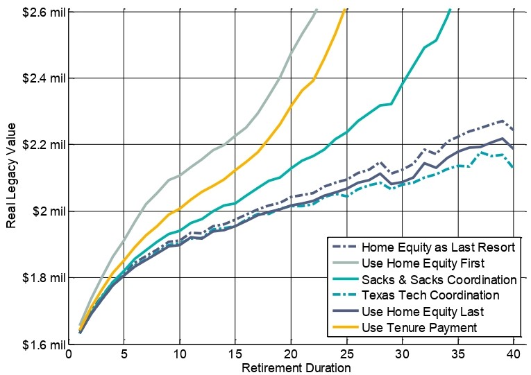
Next, Figure 3 shows the combined real legacy values at the 90th percentile of outcomes. These are cases when the investment portfolio performs extremely well throughout retirement. In these cases, what the figure demonstrates is that if one can count on outsized investment returns, there is benefit from using the line of credit more quickly, as the portfolio grows more quickly than the loan balance. Using home equity first, the tenure strategy, and the Sacks and Sacks coordination strategy all lean toward a quicker use of home equity than the other strategies, which support higher combined legacy values. Next is the last resort option, which is located where it is because of its ability to save on ever having to pay the upfront costs for a reverse mortgage that will not otherwise ever be used. The final two strategies do open the line of credit initially but end up using it very rarely if at all, and so these provide the smallest relative advantages for legacy value.
Figure 4
10th Percentile Real Legacy Value for a 4% Post-Tax Initial Withdrawal Rate
$1 million portfolio, $500,000 home value, 25% Marginal Tax Rate
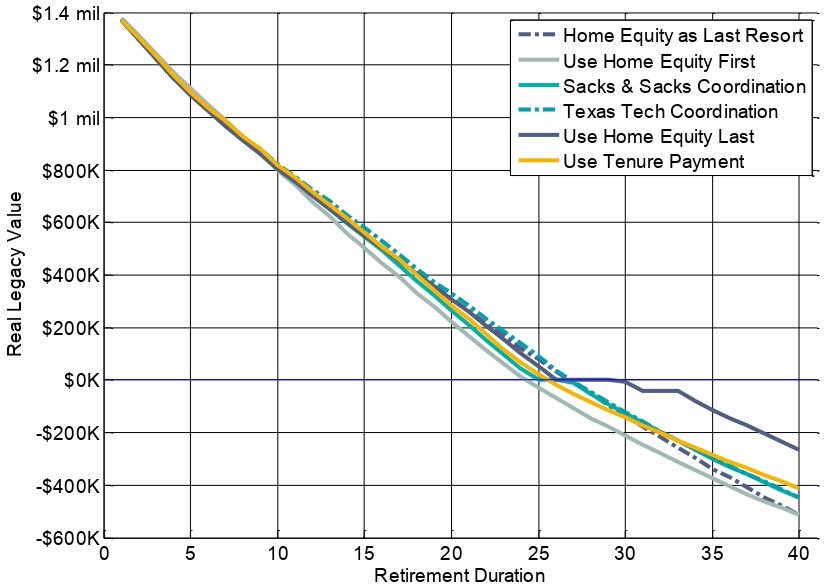
Finally, Figure 4 shows results for the 10th percentile of outcomes. These are the bad luck cases for market returns and sequence risk in which planning general focuses. In these cases, legacy values reach $0 by about 25 years in retirement. Spending down home equity first becomes the riskiest strategy, as the delay in having to start tapping the portfolio hasn’t sufficiently helped if financial markets are still significantly down a few years into retirement. Once retirements last longer, eventually, spending home equity last (after opening the line of credit early) does the best to continue supporting spending even after financial assets are depleted. For some years, there is a better chance to benefit from a line of credit which exceeds the home value, and then helps to slow the eventual portfolio shortfalls which arise once both retirement resources have been fully depleted. The tenure option also provides some income to reduce the size of shortfalls even after both resources are depleted, which happens at the 10th percentile of outcomes.
Conclusions
This article has explored six different methods for incorporating home equity into a retirement income plan through the use of a reverse mortgage. Generally, strategies which spend the home equity more quickly increase the overall risk for the retirement plan. More upside potential is generated by delaying the need to take distributions from investments, but more downside risk is created because the home equity is used quickly without necessarily being compensated by sufficiently high market returns.
Meanwhile, opening the line of credit and that start of retirement and then delaying its use until the portfolio is depleted creates the most downside protection for the retirement income plan. This strategy allows the line of credit to grow longer, perhaps surpassing the home’s value before it is used, which provides a bigger base to continue retirement spending after the portfolio is depleted. Using home equity last does reduce upside potential because when markets are strong the portfolio will grow faster than the loan balance.
Frequently, this line of credit growth opportunity serves a stronger role than the benefits from mitigating sequence risk through the use of coordinated strategies. Nonetheless, use of tenure payments or one of the coordinated strategies can also be justified as providing a middle ground which balances the upside potential of using home equity first and the downside protection of using home equity last. These coordinated strategies can occasionally provide the best outcomes for legacy in some simulated cases when they best balance the tradeoff between using home equity soon to provide relief for the portfolio, and delaying home equity use so the available line of credit is larger.
For future research, important considerations to also factor in include different retirement spending goals, different retirement tax rates, and different fee combinations for upfront cost and margin rates. Past research has already established the increased value provided by the HECM when interest rates are low and when home equity is larger relative to the portfolio size, but it would also be intriguing to further examine these factors within the broader model provided in this article. As well, it is important to note that strategies which open a line of credit and leave it unused run counter to the objectives of lenders and the government’s mortgage insurance fund. One day these opportunities may be eliminated.
References
Bengen, William P. 1994. “Determining Withdrawal Rates Using Historical Data.” Journal of Financial Planning 7, 4 (October): 171-180.
Giordano, Shelley. 2015. What’s the Deal With Reverse Mortgages? Pennington, NJ: People Tested Media.
Johnson, David W., and Zamira S. Simkins. 2014. “Retirement Trends, Current Monetary Policy, and the Reverse Mortgage Market.” Journal of Financial Planning 27 (3): 52-59.
Pfeiffer, Shaun, John R. Salter, and Harold R. Evensky. 2013. “Increasing the Sustainable Withdrawal Rate Using the Standby Reverse Mortgage.” Journal of Financial Planning 26 (12): 55-62.
Sacks, Barry H., and Stephen R. Sacks. 2012. “Reversing the Conventional Wisdom: Using Home Equity to Supplement Retirement Income.” Journal of Financial Planning 25 (2): 43-52.
Salter, John R., Shaun A. Pfeiffer, and Harold R. Evensky. 2012. “Standby Reverse Mortgages: A Risk Management Tool for Retirement Distributions.” Journal of Financial Planning 25 (8): 40-48.
Pfau, Wade D. 2014. “The Hidden Value of a Reverse Mortgage Standby Line of Credit.” Advisor Perspectives (December 9). http://www.advisorperspectives.com/articles/2014/12/09/the-hidden-value-of-a-reverse-mortgage-standby-line-of-credit
Pfeiffer, Shaun, C. Angus Schaal, and John Salter. 2014. “HECM Reverse Mortgages: Now or Last Resort?” Journal of Financial Planning 27 (5) 44–51.
Wagner, Gerald C. 2013. “The 6.0 Percent Rule.” Journal of Financial Planning 26 (12): 46-59.
Appendix on Capital Market Expectations
The capital market expectations is this article connect the historical averages from Robert Shiller’s dataset (http://www.econ.yale.edu/~shiller/data.htm) together with the current market values for inflation and interest rates. This makes allowances for the fact that interest rates and inflation are currently far from their historical averages, but it also respects historical averages and does not force returns to remain low for the entire simulated time horizon.
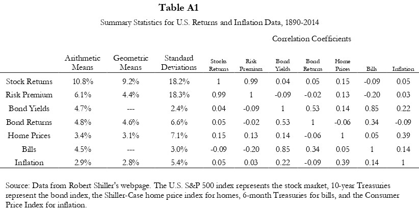
Table A1 provides summary statistics for the historical data, which guides the Monte Carlo simulations for investment returns. A Cholesky decomposition is performed on a matrix of the normalized values for the risk premium, bond yields, home prices, bills and inflation. A Monte Carlo simulation is then used to create error terms for these variables, which preserve their contemporaneous correlations with one another. Then the variables are simulated with these errors using models that preserve key characteristics about serial correlation.
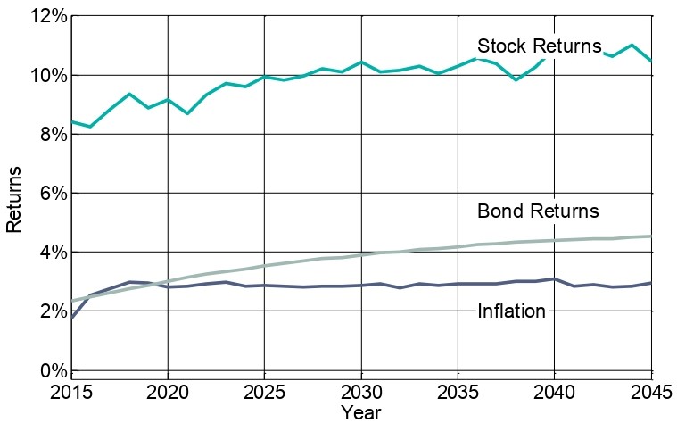
Inflation is modeled as a first order autoregressive process starting from -0.1% inflation in 2014 and trending toward its historical average over time with its historical volatility. Bond yields are similarly modeled with a first order autoregression with an initial seed value of 2%. Next, home prices and the risk premium are both modeled as random walks around their historical averages and with their historical volatilities. Bond returns are calculated from bond yields and changes in interest rates, assuming a bond mutual fund with equal holdings of past 10-year Treasury issues. Stock returns are calculated as the sum of bond yields and the equity premium over yields. LIBOR rates are calculated using corresponding Treasury rates as proxies. Figure A1 shows the medians for the key variables.
Figure A1
Medians of Simulated Outcomes for Inflation, Bonds, and Stocks